Determining Footprints from Raster Data

When creating STAC Item records from raster images, one important action is generating a spatial footprint of the image data to use for the Item geometry field. We intentionally use the imprecise term “footprint” here, as we are not trying to create a precise vector representation of the data of an image (which could contain as many polygons as pixels in the image!), but we are trying to do better than just a bounding box of the entire image, both data and no data. By footprint, we mean a vector that balances many competing factors, and generally represents a shape covering the data in an image. Figuring out the right parameter values to the methods in the raster_footprint module will usually require some experimental validation, to find exactly the right values for your data, CRS, and use cases.

There are a few properties we’d like to have in a footprint:

1. The footprint only covers the area on the image only where there is data.

2. The footprint has enough points to accurately capture the shape of the data in the EPSG:4326 CRS used by GeoJSON.

3. The footprint does not have too many points, such that it is becomes very large.

Discussion of these properties follows.

Only Data Areas are Represented

Typically, gridded imagery will have image files representing a single grid square, with no data values where there is no data. There are many reasons why an image may contain no data values, and we will describe a few of them here.

In the Sentinel-2 L2A product, many images only have a partial swath of data where an orbit of the sensor only captured data within part of a single grid square.

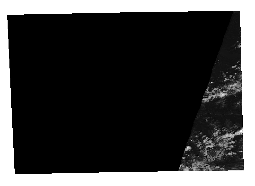
Ideally, our footprint generated from this image would not cover the entire image, but only the area where there is data, like this:

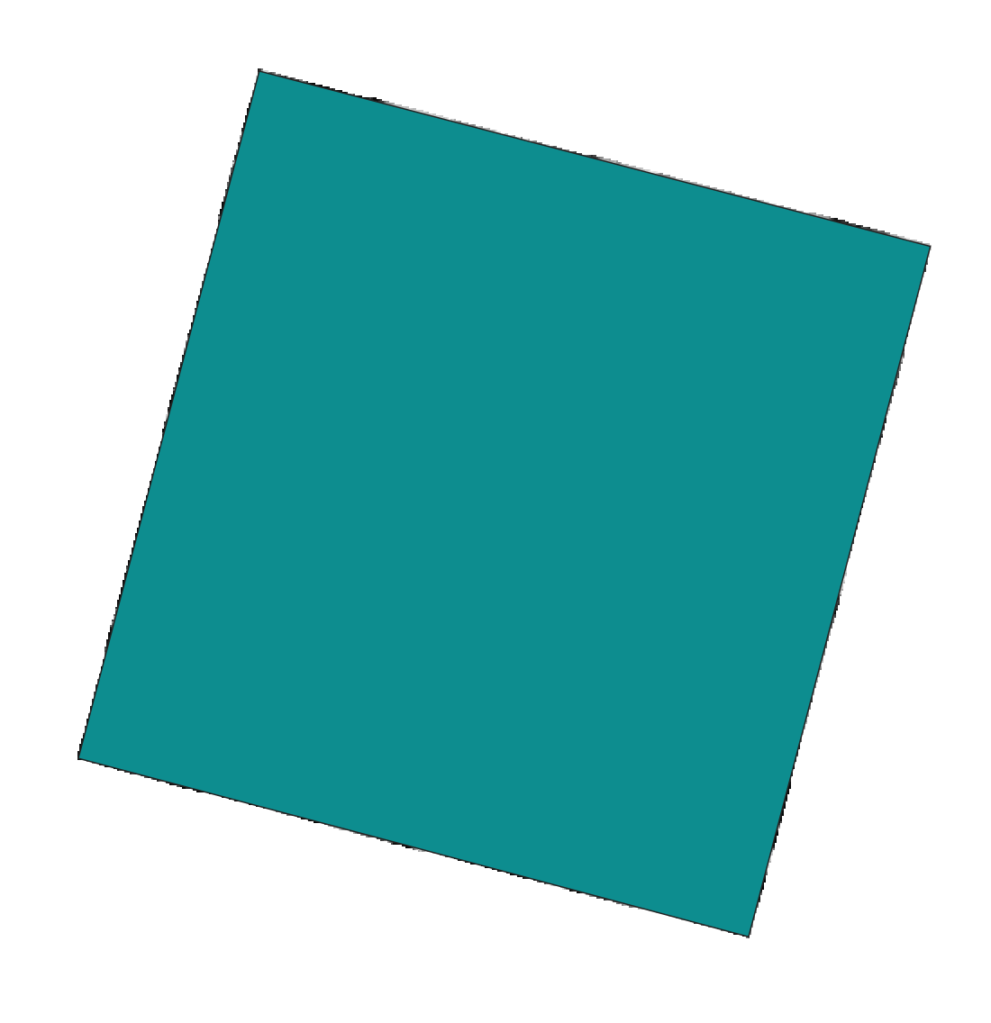
In the Landsat 8 product, the data area appears rotated, as the orbit of the satellite and path-row gridding is not aligned with the CRS.

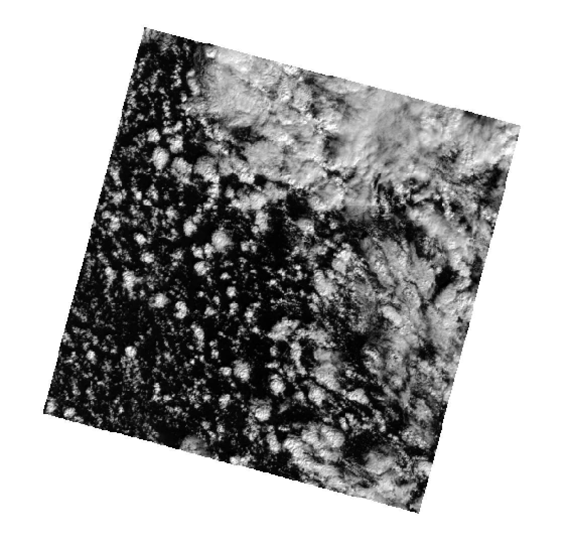
We’d like the footprint to only cover that data area, and not the no data areas that square the image:

Another issue is products that use no data values for areas where clouds, snow, or ice exist. A precise vector representation of such an image would likely be a MultiPolygon with holes where the no data values are. However, this is rarely useful for STAC use cases.

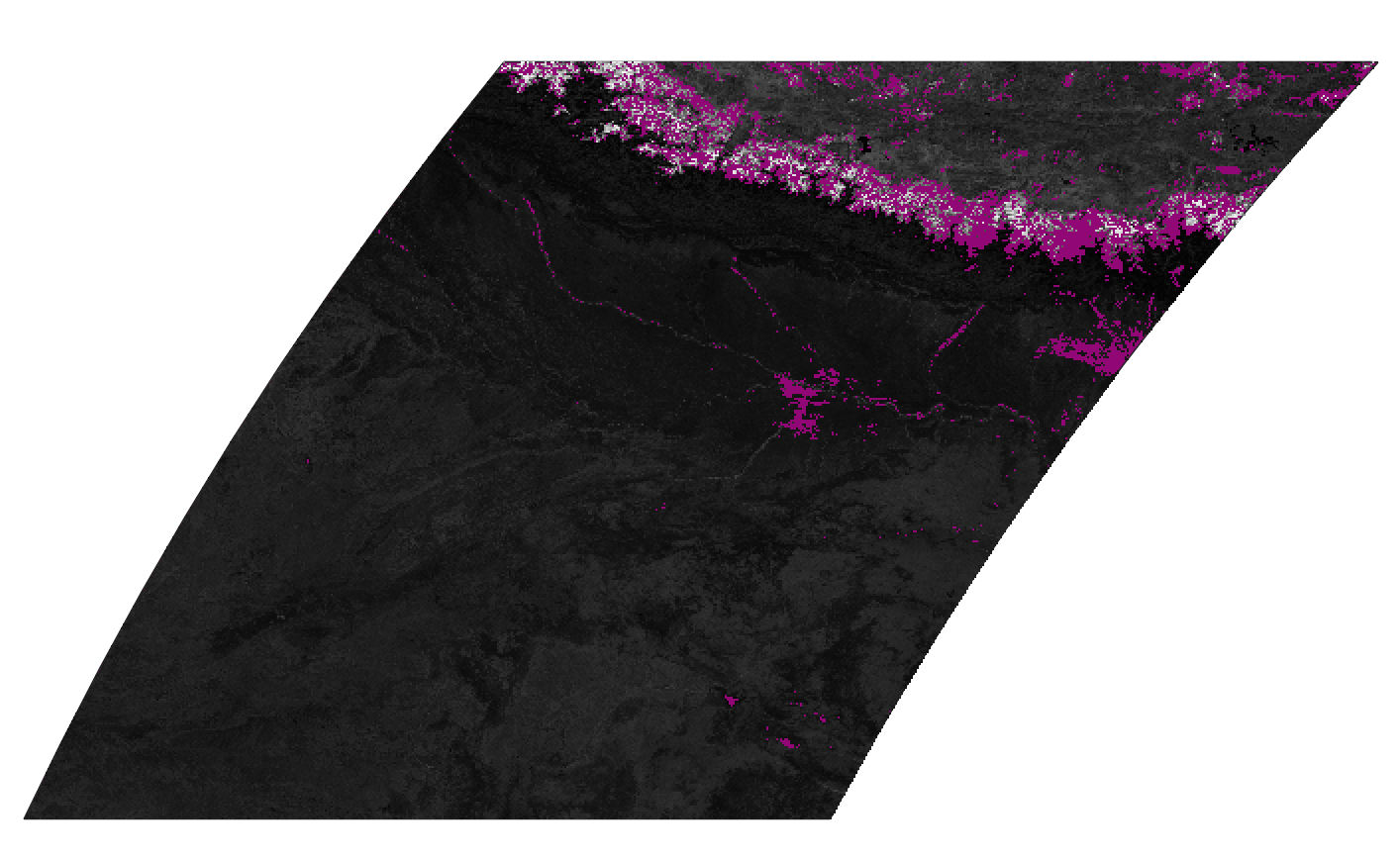
Likewise, where an area of no data values coincide with one of of the edges of the image, we could attempt to create a concavity to carve out the no data pixels through the calculation of the alpha shape. Instead, we take an easier approach and create a convex hull around the data areas of the image. In practice, the difference in coverage between the convex hull and the alpha shape is relatively small. This difference has the potential to result in false positives where a search geometry intersects the geometry of an Item, but the only pixels within the geometry are no data, but in practice this is rarely a problem.

When using the raster_footprint functions, the no_data parameter value can be used to pass in the value used for no data if it is not defined in the image metadata.

Reprojected Geometry Accurately Represents the Footprint

In the native CRS, the geometry of the data area of an image can typically be represented by a polygon containing a small number of points. If the entire image has data pixels, it maybe represented by a 5 point polygon (where the first and last points are the same). When this polygon is reprojected to EPSG:4326, it will still result in a 5 point polygon, as the points have simply been reprojected into the new CRS. This new polygon may not accurately represent original polygon if there is significant curved distortion between the CRSs. An example of this is most apparent in reprojecting the sinusoidal geometry of MODIS to EPSG:4326. Simply reprojecting the 5 point polygon would result in a parallelogram, whereas a more accurate representation is two parallel straight sides and two curved sides.

To increase the accuracy of the reprojected shape, we can first densify the polygon. Here we add additional, redundant points between existing points in the polygon, so that the reprojected shape will have points that more closely match the actual form of the reprojection. In the above example for MODIS, we have used a densification factor of 10, so that each “side” of the polygon has 11 points representing it instead of 2, and we get a “curved” side that more closely matches the raster reprojection.

When using the methods in the raster_footprint module, the densification_factor or densification_distance parameter can be used to densify the geometry before reprojection. This will require some experimentation to find the appropriate value for the CRS of your data.

Simplifying the Geometry

A 4801 point polygon is required to precisely represent a MODIS tile in EPSG:4326 to accurately represent itself, as it is a 2400x2400 pixel image and two sides are curves after reprojection. However, a polygon this dense both makes the Item body very large and increases the computation required to perform an intersects calculation during search, with little benefit. These polygons can be simplified by defining a maximum distance, in degrees, within which the simplified polygon must be to original polygon points. This is also useful when the polygon in the native CRS has a large number of points, so that the end result is a polygon of a more manageable size.

When using the methods in the raster_footprint module, the simplify_tolerance parameter defines the distance within which the simplified polygon must be to the original polygon points. This will require some experimentation to find the appropriate value for the CRS of your data.